Datatypes of programming languages

Uncategorized

Fourth Normal Form (4NF)

Database Concept

DBMS ER Model

DBMS Relational model

DBMS Normalization

DBMS Basic SQL

DBMS DML Command

DBMS DCL Command

Advanced SQL

Fourth Normal Form comes into picture when Multi-valued Dependency occur in any relation. In this tutorial we will learn about Multi-valued Dependency, how to remove it and how to make any table satisfy the fourth normal form.

Follow the video above for complete explanation of 4th Normal Form. Or, if you want, you can even skip the video and jump to the section below for the complete tutorial.

In our last tutorial, we learned about the boyce-codd normal form, we suggest you to follow the last tutorial before this one.

Rules for 4th Normal Form

For a table to satisfy the Fourth Normal Form, it should satisfy the following two conditions:

It should be in the Boyce-Codd Normal Form.
And, the table should not have any Multi-valued Dependency.

Let’s try to understand what multi-valued dependency is in the next section.

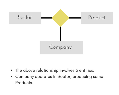
What is Multi-valued Dependency?

A table is said to have multi-valued dependency, if the following conditions are true,

For a dependency A → B, if for a single value of A, multiple value of B exists, then the table may have multi-valued dependency.
Also, a table should have at-least 3 columns for it to have a multi-valued dependency.
And, for a relation R(A,B,C), if there is a multi-valued dependency between, A and B, then B and C should be independent of each other.

If all these conditions are true for any relation(table), it is said to have multi-valued dependency.

Time for an Example

Below we have a college enrolment table with columns s_id, course and hobby.

s_id	course	hobby
1	Science	Cricket
1	Maths	Hockey
2	C#	Cricket
2	Php	Hockey

As you can see in the table above, student with s_id 1 has opted for two courses, Science and Maths, and has two hobbies, Cricket and Hockey.

You must be thinking what problem this can lead to, right?

Well the two records for student with s_id 1, will give rise to two more records, as shown below, because for one student, two hobbies exists, hence along with both the courses, these hobbies should be specified.

s_id	course	hobby
1	Science	Cricket
1	Maths	Hockey
1	Science	Hockey
1	Maths	Cricket

And, in the table above, there is no relationship between the columns course and hobby. They are independent of each other.

So there is multi-value dependency, which leads to un-necessary repetition of data and other anomalies as well.

How to satisfy 4th Normal Form?

To make the above relation satify the 4th normal form, we can decompose the table into 2 tables.

CourseOpted Table

s_id	course
1	Science
1	Maths
2	C#
2	Php

And, Hobbies Table,

s_id	hobby
1	Cricket
1	Hockey
2	Cricket
2	Hockey

Now this relation satisfies the fourth normal form.

A table can also have functional dependency along with multi-valued dependency. In that case, the functionally dependent columns are moved in a separate table and the multi-valued dependent columns are moved to separate tables.

If you design your database carefully, you can easily avoid these issues.

< prev

Next >

Uncategorized

What is Relational Calculus?

Database Concept

DBMS ER Model

DBMS Relational model

DBMS Normalization

DBMS Basic SQL

DBMS DML Command

DBMS DCL Command

Advanced SQL

Contrary to Relational Algebra which is a procedural query language to fetch data and which also explains how it is done, Relational Calculus in non-procedural query language and has no description about how the query will work or the data will b fetched. It only focusses on what to do, and not on how to do it.

Relational Calculus exists in two forms:

Tuple Relational Calculus (TRC)
Domain Relational Calculus (DRC)

Tuple Relational Calculus (TRC)

In tuple relational calculus, we work on filtering tuples based on the given condition.

Syntax: { T | Condition }

In this form of relational calculus, we define a tuple variable, specify the table(relation) name in which the tuple is to be searched for, along with a condition.

We can also specify column name using a . dot operator, with the tuple variable to only get a certain attribute(column) in result.

A lot of informtion, right! Give it some time to sink in.

A tuple variable is nothing but a name, can be anything, generally we use a single alphabet for this, so let’s say T is a tuple variable.

To specify the name of the relation(table) in which we want to look for data, we do the following:

Relation(T), where T is our tuple variable.

For example if our table is Student, we would put it as Student(T)

Then comes the condition part, to specify a condition applicable for a particluar attribute(column), we can use the . dot variable with the tuple variable to specify it, like in table Student, if we want to get data for students with age greater than 17, then, we can write it as,

T.age > 17, where T is our tuple variable.

Putting it all together, if we want to use Tuple Relational Calculus to fetch names of students, from table Student, with age greater than 17, then, for T being our tuple variable,

T.name | Student(T) AND T.age > 17

Domain Relational Calculus (DRC)

In domain relational calculus, filtering is done based on the domain of the attributes and not based on the tuple values.

Syntax: { c1, c2, c3, ..., cn | F(c1, c2, c3, ... ,cn)}

where, c1, c2… etc represents domain of attributes(columns) and F defines the formula including the condition for fetching the data.

For example,

{< name, age > | ∈ Student ∧ age > 17}

Again, the above query will return the names and ages of the students in the table Student who are older than 17

< prev

Next >

Uncategorized

Working with ER Diagrams

Database Concept

DBMS ER Model

DBMS Relational model

DBMS Normalization

DBMS Basic SQL

DBMS DML Command

DBMS DCL Command

Advanced SQL

ER Diagram is a visual representation of data that describes how data is related to each other. In ER Model, we disintegrate data into entities, attributes and setup relationships between entities, all this can be represented visually using the ER diagram.

For example, in the below diagram, anyone can see and understand what the diagram wants to convey: Developer develops a website, whereas a Visitor visits a website.

Components of ER Diagram

Entitiy, Attributes, Relationships etc form the components of ER Diagram and there are defined symbols and shapes to represent each one of them.

Let’s see how we can represent these in our ER Diagram.

Entity

Simple rectangular box represents an Entity.

Relationships between Entities – Weak and Strong

Rhombus is used to setup relationships between two or more entities.

Attributes for any Entity

Ellipse is used to represent attributes of any entity. It is connected to the entity.

Weak Entity

A weak Entity is represented using double rectangular boxes. It is generally connected to another entity.

Key Attribute for any Entity

To represent a Key attribute, the attribute name inside the Ellipse is underlined.

Derived Attribute for any Entity

Derived attributes are those which are derived based on other attributes, for example, age can be derived from date of birth.To represent a derived attribute, another dotted ellipse is created inside the main ellipse.

Multivalued Attribute for any Entity

Double Ellipse, one inside another, represents the attribute which can have multiple values.

Composite Attribute for any Entity

A composite attribute is the attribute, which also has attributes.

ER Diagram: Entity

An Entity can be any object, place, person or class. In ER Diagram, an entity is represented using rectangles. Consider an example of an Organisation- Employee, Manager, Department, Product and many more can be taken as entities in an Organisation.

The yellow rhombus in between represents a relationship.

ER Diagram: Weak Entity

Weak entity is an entity that depends on another entity. Weak entity doesn’t have anay key attribute of its own. Double rectangle is used to represent a weak entity.

ER Diagram: Attribute

An Attribute describes a property or characterstic of an entity. For example, Name, Age, Address etc can be attributes of a Student. An attribute is represented using eclipse.

ER Diagram: Key Attribute

Key attribute represents the main characterstic of an Entity. It is used to represent a Primary key. Ellipse with the text underlined, represents Key Attribute.

ER Diagram: Composite Attribute

An attribute can also have their own attributes. These attributes are known as Composite attributes.

ER Diagram: Relationship

A Relationship describes relation between entities. Relationship is represented using diamonds or rhombus.

There are three types of relationship that exist between Entities.

Binary Relationship
Recursive Relationship
Ternary Relationship

ER Diagram: Binary Relationship

Binary Relationship means relation between two Entities. This is further divided into three types.

One to One Relationship

This type of relationship is rarely seen in real world.

The above example describes that one student can enroll only for one course and a course will also have only one Student. This is not what you will usually see in real-world relationships.

One to Many Relationship

The below example showcases this relationship, which means that 1 student can opt for many courses, but a course can only have 1 student. Sounds weird! This is how it is.

Many to One Relationship

It reflects business rule that many entities can be associated with just one entity. For example, Student enrolls for only one Course but a Course can have many Students.

Many to Many Relationship

The above diagram represents that one student can enroll for more than one courses. And a course can have more than 1 student enrolled in it.

ER Diagram: Recursive Relationship

When an Entity is related with itself it is known as Recursive Relationship.

recursive relationship example ER diagram

ER Diagram: Ternary Relationship

Relationship of degree three is called Ternary relationship.

A Ternary relationship involves three entities. In such relationships we always consider two entites together and then look upon the third.

For example, in the diagram above, we have three related entities, Company, Product and Sector. To understand the relationship better or to define rules around the model, we should relate two entities and then derive the third one.

A Company produces many Products/ each product is produced by exactly one company.

A Company operates in only one Sector / each sector has many companies operating in it.

Considering the above two rules or relationships, we see that although the complete relationship involves three entities, but we are looking at two entities at a time.

< prev

Next >

Uncategorized

Understanding DBMS Architecture

Database Concept

DBMS ER Model

DBMS Relational model

DBMS Normalization

DBMS Basic SQL

DBMS DML Command

DBMS DCL Command

Advanced SQL

A Database Management system is not always directly available for users and applications to access and store data in it. A Database Management system can be centralised(all the data stored at one location), decentralised(multiple copies of database at different locations) or hierarchical, depending upon its architecture.

1-tier DBMS architecture also exist, this is when the database is directly available to the user for using it to store data. Generally such a setup is used for local application development, where programmers communicate directly with the database for quick response.

Database Architecture is logically of two types:

2-tier DBMS architecture
3-tier DBMS architecture

2-tier DBMS Architecture

2-tier DBMS architecture includes an Application layer between the user and the DBMS, which is responsible to communicate the user’s request to the database management system and then send the response from the DBMS to the user.

An application interface known as ODBC(Open Database Connectivity) provides an API that allow client side program to call the DBMS. Most DBMS vendors provide ODBC drivers for their DBMS.

Such an architecture provides the DBMS extra security as it is not exposed to the End User directly. Also, security can be improved by adding security and authentication checks in the Application layer too.

3-tier DBMS Architecture

3-tier DBMS architecture is the most commonly used architecture for web applications.

It is an extension of the 2-tier architecture. In the 2-tier architecture, we have an application layer which can be accessed programatically to perform various operations on the DBMS. The application generally understands the Database Access Language and processes end users requests to the DBMS.

In 3-tier architecture, an additional Presentation or GUI Layer is added, which provides a graphical user interface for the End user to interact with the DBMS.

For the end user, the GUI layer is the Database System, and the end user has no idea about the application layer and the DBMS system.

If you have used MySQL, then you must have seen PHPMyAdmin, it is the best example of a 3-tier DBMS architecture.

< prev

Next >

C++, programming languages

C++ Type Conversion

C++ Tutorial

C++ Introduction

C++ Flow Control

C++ Functions

C++ Arrays & String

C++ Structures

C++ Object & Class

C++ Pointers

C++ Inheritance

In this tutorial, we will learn about the basics of C++ type conversion with the help of examples.

C++ allows us to convert data of one type to that of another. This is known as type conversion.

There are two types of type conversion in C++.

Implicit Conversion
Explicit Conversion (also known as Type Casting)

Implicit Type Conversion

The type conversion that is done automatically done by the compiler is known as implicit type conversion. This type of conversion is also known as automatic conversion.

Let us look at two examples of implicit type conversion.

Example 1: Conversion From int to double

// Working of implicit type-conversion

#include <iostream>
using namespace std;

int main() {
   // assigning an int value to num_int
   int num_int = 9;

   // declaring a double type variable
   double num_double;
 
   // implicit conversion
   // assigning int value to a double variable
   num_double = num_int;

   cout << "num_int = " << num_int << endl;
   cout << "num_double = " << num_double << endl;

   return 0;
}

Run Code

Output

num_int = 9
num_double = 9

In the program, we have assigned an int data to a double variable.

num_double = num_int;

Here, the int value is automatically converted to double by the compiler before it is assigned to the num_double variable. This is an example of implicit type conversion.

Example 2: Automatic Conversion from double to int

//Working of Implicit type-conversion

#include <iostream>
using namespace std;

int main() {

   int num_int;
   double num_double = 9.99;

   // implicit conversion
   // assigning a double value to an int variable
   num_int = num_double;

   cout << "num_int = " << num_int << endl;
   cout << "num_double = " << num_double << endl;

   return 0;
}

Run Code

Output

num_int = 9
num_double = 9.99

In the program, we have assigned a double data to an int variable.

num_double = num_int;

Here, the double value is automatically converted to int by the compiler before it is assigned to the num_int variable. This is also an example of implicit type conversion.

Note: Since int cannot have a decimal part, the digits after the decimal point is truncated in the above example.

Data Loss During Conversion (Narrowing Conversion)

As we have seen from the above example, conversion from one data type to another is prone to data loss. This happens when data of a larger type is converted to data of a smaller type.

Data loss in C++ if a larger type of data is converted to a smaller type. — Possible Data Loss During Type Conversion

C++ Explicit Conversion

When the user manually changes data from one type to another, this is known as explicit conversion. This type of conversion is also known as type casting.

There are three major ways in which we can use explicit conversion in C++. They are:

C-style type casting (also known as cast notation)
Function notation (also known as old C++ style type casting)
Type conversion operators

C-style Type Casting

As the name suggests, this type of casting is favored by the C programming language. It is also known as cast notation.

The syntax for this style is:

(data_type)expression;

For example,

// initializing int variable
int num_int = 26;

// declaring double variable
double num_double;

// converting from int to double
num_double = (double)num_int;

Function-style Casting

We can also use the function like notation to cast data from one type to another.

The syntax for this style is:

data_type(expression);

For example,

// initializing int variable
int num_int = 26;

// declaring double variable
double num_double;

// converting from int to double
num_double = double(num_int);

Example 3: Type Casting

#include <iostream>

using namespace std;

int main() {
    // initializing a double variable
    double num_double = 3.56;
    cout << "num_double = " << num_double << endl;

    // C-style conversion from double to int
    int num_int1 = (int)num_double;
    cout << "num_int1   = " << num_int1 << endl;

    // function-style conversion from double to int
    int num_int2 = int(num_double);
    cout << "num_int2   = " << num_int2 << endl;

    return 0;
}

Run Code

Output

num_double = 3.56
num_int1   = 3
num_int2   = 3

We used both the C style type conversion and the function-style casting for type conversion and displayed the results. Since they perform the same task, both give us the same output.

Type Conversion Operators

Besides these two type castings, C++ also has four operators for type conversion. They are known as type conversion operators. They are:

static_cast
dynamic_cast
const_cast
reinterpret_cast

We will learn about these casts in later tutorials.

Recommended Tutorials:

C++ string to int and Vice-versa
C++ string to float, double and Vice-versa

< prev

next >

c, programming languages

C Datatype

In this tutorial, you will learn about basic data types such as int, float, char etc. in C programming.

In C programming, data types are declarations for variables. This determines the type and size of data associated with variables. For example,

int myVar;

Here, myVar is a variable of int (integer) type. The size of int is 4 bytes.

Basic types

Here’s a table containing commonly used types in C programming for quick access.

Type	Size (bytes)	Format Specifier
`int`	at least 2, usually 4	`%d`, `%i`
`char`	1	`%c`
`float`	4	`%f`
`double`	8	`%lf`
`short int`	2 usually	`%hd`
`unsigned int`	at least 2, usually 4	`%u`
`long int`	at least 4, usually 8	`%ld`, `%li`
`long long int`	at least 8	`%lld`, `%lli`
`unsigned long int`	at least 4	`%lu`
`unsigned long long int`	at least 8	`%llu`
`signed char`	1	`%c`
`unsigned char`	1	`%c`
`long double`	at least 10, usually 12 or 16	`%Lf`

int

Integers are whole numbers that can have both zero, positive and negative values but no decimal values. For example, 0, -5, 10

We can use int for declaring an integer variable.

int id;

Here, id is a variable of type integer.

You can declare multiple variables at once in C programming. For example,

int id, age;

The size of int is usually 4 bytes (32 bits). And, it can take 2³² distinct states from -2147483648 to 2147483647.

float and double

float and double are used to hold real numbers.

float salary;
double price;

In C, floating-point numbers can also be represented in exponential. For example,

float normalizationFactor = 22.442e2;

What’s the difference between float and double?

The size of float (single precision float data type) is 4 bytes. And the size of double (double precision float data type) is 8 bytes.

char

Keyword char is used for declaring character type variables. For example,

char test = 'h';

The size of the character variable is 1 byte.

void

void is an incomplete type. It means “nothing” or “no type”. You can think of void as absent.

For example, if a function is not returning anything, its return type should be void.

Note that, you cannot create variables of void type.

short and long

If you need to use a large number, you can use a type specifier long. Here’s how:

long a;
long long b;
long double c;

Here variables a and b can store integer values. And, c can store a floating-point number.

If you are sure, only a small integer ([−32,767, +32,767] range) will be used, you can use short.

short d;

You can always check the size of a variable using the sizeof() operator.

#include <stdio.h>      
int main() {
  short a;
  long b;
  long long c;
  long double d;

  printf("size of short = %d bytes\n", sizeof(a));
  printf("size of long = %d bytes\n", sizeof(b));
  printf("size of long long = %d bytes\n", sizeof(c));
  printf("size of long double= %d bytes\n", sizeof(d));
  return 0;
}

signed and unsigned

In C, signed and unsigned are type modifiers. You can alter the data storage of a data type by using them. For example,

unsigned int x;
int y;

Here, the variable x can hold only zero and positive values because we have used the unsigned modifier.

Considering the size of int is 4 bytes, variable y can hold values from -2³¹ to 2³¹-1, whereas variable x can hold values from 0 to 2³²-1.

Other data types defined in C programming are:

bool Type
Enumerated type
Complex types

Derived Data Types

Data types that are derived from fundamental data types are derived types. For example: arrays, pointers, function types, structures, etc.

We will learn about these derived data types in later tutorials.

< prev

Next >