Boyce-Codd Normal Form or BCNF is an extension to the third normal form, and is also known as 3.5 Normal Form.
Follow the video above for complete explanation of BCNF. Or, if you want, you can even skip the video and jump to the section below for the complete tutorial.
In our last tutorial, we learned about the third normal form and we also learned how to remove transitive dependency from a table, we suggest you to follow the last tutorial before this one.
Rules for BCNF
For a table to satisfy the Boyce-Codd Normal Form, it should satisfy the following two conditions:
It should be in the Third Normal Form.
And, for any dependency A → B, A should be a super key.
The second point sounds a bit tricky, right? In simple words, it means, that for a dependency A → B, A cannot be a non-prime attribute, if B is a prime attribute.
Time for an Example
Below we have a college enrolment table with columns student_id, subject and professor.
student_id
subject
professor
101
Java
P.Java
101
C++
P.Cpp
102
Java
P.Java2
103
C#
P.Chash
104
Java
P.Java
As you can see, we have also added some sample data to the table.
In the table above:
One student can enrol for multiple subjects. For example, student with student_id 101, has opted for subjects – Java & C++
For each subject, a professor is assigned to the student.
And, there can be multiple professors teaching one subject like we have for Java.
What do you think should be the Primary Key?
Well, in the table above student_id, subject together form the primary key, because using student_id and subject, we can find all the columns of the table.
One more important point to note here is, one professor teaches only one subject, but one subject may have two different professors.
Hence, there is a dependency between subject and professor here, where subject depends on the professor name.
This table satisfies the 1st Normal form because all the values are atomic, column names are unique and all the values stored in a particular column are of same domain.
This table also satisfies the 2nd Normal Form as their is no Partial Dependency.
And, there is no Transitive Dependency, hence the table also satisfies the 3rd Normal Form.
But this table is not in Boyce-Codd Normal Form.
Why this table is not in BCNF?
In the table above, student_id, subject form primary key, which means subject column is a prime attribute.
But, there is one more dependency, professor → subject.
And while subject is a prime attribute, professor is a non-prime attribute, which is not allowed by BCNF.
To make this relation(table) satisfy BCNF, we will decompose this table into two tables, student table and professor table.
Below we have the structure for both the tables.
Student Table
student_id
p_id
101
1
101
2
and so on…
And, Professor Table
p_id
professor
subject
1
P.Java
Java
2
P.Cpp
C++
and so on…
And now, this relation satisfy Boyce-Codd Normal Form. In the next tutorial we will learn about the Fourth Normal Form.
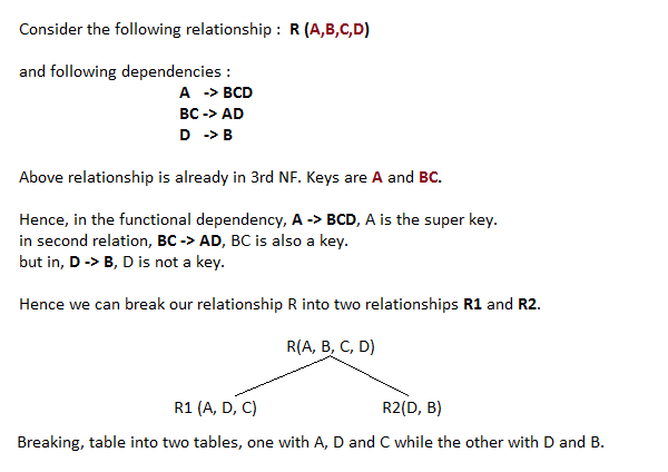
A more Generic Explanation
In the picture below, we have tried to explain BCNF in terms of relations.
For a table to be in the Second Normal Form, it must satisfy two conditions:
The table should be in the First Normal Form.
There should be no Partial Dependency.
If you want you can skip the video, as the concept is covered in detail below the video.
What is Partial Dependency? Do not worry about it. First let’s understand what is Dependency in a table?
What is Dependency?
Let’s take an example of a Student table with columns student_id, name, reg_no(registration number), branch and address(student’s home address).
student_id
name
reg_no
branch
address
In this table, student_id is the primary key and will be unique for every row, hence we can use student_id to fetch any row of data from this table
Even for a case, where student names are same, if we know the student_id we can easily fetch the correct record.
student_id
name
reg_no
branch
address
10
Akon
07-WY
CSE
Kerala
11
Akon
08-WY
IT
Gujarat
Hence we can say a Primary Key for a table is the column or a group of columns(composite key) which can uniquely identify each record in the table.
I can ask from branch name of student with student_id10, and I can get it. Similarly, if I ask for name of student with student_id10 or 11, I will get it. So all I need is student_id and every other column depends on it, or can be fetched using it.
This is Dependency and we also call it Functional Dependency.
What is Partial Dependency?
Now that we know what dependency is, we are in a better state to understand what partial dependency is.
For a simple table like Student, a single column like student_id can uniquely identfy all the records in a table.
But this is not true all the time. So now let’s extend our example to see if more than 1 column together can act as a primary key.
Let’s create another table for Subject, which will have subject_id and subject_name fields and subject_id will be the primary key.
subject_id
subject_name
1
Java
2
C++
3
Php
Now we have a Student table with student information and another table Subject for storing subject information.
Let’s create another table Score, to store the marks obtained by students in the respective subjects. We will also be saving name of the teacher who teaches that subject along with marks.
score_id
student_id
subject_id
marks
teacher
1
10
1
70
Java Teacher
2
10
2
75
C++ Teacher
3
11
1
80
Java Teacher
In the score table we are saving the student_id to know which student’s marks are these and subject_id to know for which subject the marks are for.
Together, student_id + subject_id forms a Candidate Key(learn about Database Keys) for this table, which can be the Primary key.
Confused, How this combination can be a primary key?
See, if I ask you to get me marks of student with student_id 10, can you get it from this table? No, because you don’t know for which subject. And if I give you subject_id, you would not know for which student. Hence we need student_id + subject_id to uniquely identify any row.
But where is Partial Dependency?
Now if you look at the Score table, we have a column names teacher which is only dependent on the subject, for Java it’s Java Teacher and for C++ it’s C++ Teacher & so on.
Now as we just discussed that the primary key for this table is a composition of two columns which is student_id & subject_id but the teacher’s name only depends on subject, hence the subject_id, and has nothing to do with student_id.
This is Partial Dependency, where an attribute in a table depends on only a part of the primary key and not on the whole key.
How to remove Partial Dependency?
There can be many different solutions for this, but out objective is to remove teacher’s name from Score table.
The simplest solution is to remove columns teacher from Score table and add it to the Subject table. Hence, the Subject table will become:
subject_id
subject_name
teacher
1
Java
Java Teacher
2
C++
C++ Teacher
3
Php
Php Teacher
And our Score table is now in the second normal form, with no partial dependency.
score_id
student_id
subject_id
marks
1
10
1
70
2
10
2
75
3
11
1
80
Quick Recap
For a table to be in the Second Normal form, it should be in the First Normal form and it should not have Partial Dependency.
Partial Dependency exists, when for a composite primary key, any attribute in the table depends only on a part of the primary key and not on the complete primary key.
To remove Partial dependency, we can divide the table, remove the attribute which is causing partial dependency, and move it to some other table where it fits in well.
As we all know that ER Model can be represented using ER Diagrams which is a great way of designing and representing the database design in more of a flow chart form.
It is very convenient to design the database using the ER Model by creating an ER diagram and later on converting it into relational model to design your tables.
Not all the ER Model constraints and components can be directly transformed into relational model, but an approximate schema can be derived.
So let’s take a few examples of ER diagrams and convert it into relational model schema, hence creating tables in RDBMS.
Entity becomes Table
Entity in ER Model is changed into tables, or we can say for every Entity in ER model, a table is created in Relational Model.
And the attributes of the Entity gets converted to columns of the table.
And the primary key specified for the entity in the ER model, will become the primary key for the table in relational model.
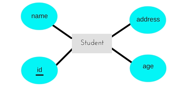
For example, for the below ER Diagram in ER Model,
A table with name Student will be created in relational model, which will have 4 columns, id, name, age, address and id will be the primary key for this table.
Relationship becomes a Relationship Table
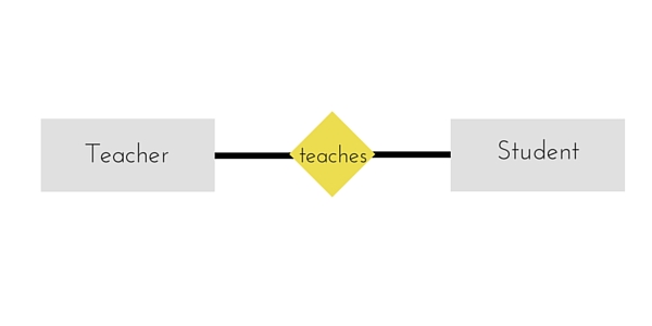
In ER diagram, we use diamond/rhombus to reprsent a relationship between two entities. In Relational model we create a relationship table for ER Model relationships too.
In the ER diagram below, we have two entities Teacher and Student with a relationship between them.
As discussd above, entity gets mapped to table, hence we will create table for Teacher and a table for Student with all the attributes converted into columns.
Now, an additional table will be created for the relationship, for example StudentTeacher or give it any name you like. This table will hold the primary key for both Student and Teacher, in a tuple to describe the relationship, which teacher teaches which student.
If there are additional attributes related to this relationship, then they become the columns for this table, like subject name.
Also proper foriegn key constraints must be set for all the tables.
Points to Remember
Similarly we can generate relational database schema using the ER diagram. Following are some key points to keep in mind while doing so:
Entity gets converted into Table, with all the attributes becoming fields(columns) in the table.
Relationship between entities is also converted into table with primary keys of the related entities also stored in it as foreign keys.
Primary Keys should be properly set.
For any relationship of Weak Entity, if primary key of any other entity is included in a table, foriegn key constraint must be defined.
Contrary to Relational Algebra which is a procedural query language to fetch data and which also explains how it is done, Relational Calculus in non-procedural query language and has no description about how the query will work or the data will b fetched. It only focusses on what to do, and not on how to do it.
Relational Calculus exists in two forms:
Tuple Relational Calculus (TRC)
Domain Relational Calculus (DRC)
Tuple Relational Calculus (TRC)
In tuple relational calculus, we work on filtering tuples based on the given condition.
Syntax:{ T | Condition }
In this form of relational calculus, we define a tuple variable, specify the table(relation) name in which the tuple is to be searched for, along with a condition.
We can also specify column name using a . dot operator, with the tuple variable to only get a certain attribute(column) in result.
A lot of informtion, right! Give it some time to sink in.
A tuple variable is nothing but a name, can be anything, generally we use a single alphabet for this, so let’s say T is a tuple variable.
To specify the name of the relation(table) in which we want to look for data, we do the following:
Relation(T), where T is our tuple variable.
For example if our table is Student, we would put it as Student(T)
Then comes the condition part, to specify a condition applicable for a particluar attribute(column), we can use the . dot variable with the tuple variable to specify it, like in table Student, if we want to get data for students with age greater than 17, then, we can write it as,
T.age > 17, where T is our tuple variable.
Putting it all together, if we want to use Tuple Relational Calculus to fetch names of students, from table Student, with age greater than 17, then, for T being our tuple variable,
T.name | Student(T) AND T.age > 17
Domain Relational Calculus (DRC)
In domain relational calculus, filtering is done based on the domain of the attributes and not based on the tuple values.
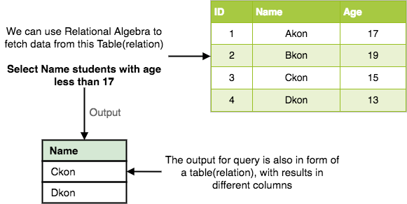
Every database management system must define a query language to allow users to access the data stored in the database. Relational Algebra is a procedural query language used to query the database tables to access data in different ways.
In relational algebra, input is a relation(table from which data has to be accessed) and output is also a relation(a temporary table holding the data asked for by the user).
Relational Algebra works on the whole table at once, so we do not have to use loops etc to iterate over all the rows(tuples) of data one by one. All we have to do is specify the table name from which we need the data, and in a single line of command, relational algebra will traverse the entire given table to fetch data for you.
The primary operations that we can perform using relational algebra are:
Select
Project
Union
Set Different
Cartesian product
Rename
Select Operation (σ)
This is used to fetch rows(tuples) from table(relation) which satisfies a given condition.
Syntax:σp(r)
Where, σ represents the Select Predicate, r is the name of relation(table name in which you want to look for data), and p is the prepositional logic, where we specify the conditions that must be satisfied by the data. In prepositional logic, one can use unary and binary operators like =, <, > etc, to specify the conditions.
Let’s take an example of the Student table we specified above in the Introduction of relational algebra, and fetch data for students with age more than 17.
σage > 17 (Student)
This will fetch the tuples(rows) from table Student, for which age will be greater than 17.
You can also use, and, or etc operators, to specify two conditions, for example,
σage > 17 and gender = 'Male' (Student)
This will return tuples(rows) from table Student with information of male students, of age more than 17.(Consider the Student table has an attribute Gender too.)
Project Operation (∏)
Project operation is used to project only a certain set of attributes of a relation. In simple words, If you want to see only the names all of the students in the Student table, then you can use Project Operation.
It will only project or show the columns or attributes asked for, and will also remove duplicate data from the columns.
Syntax:∏A1, A2...(r)
where A1, A2 etc are attribute names(column names).
For example,
∏Name, Age(Student)
Above statement will show us only the Name and Age columns for all the rows of data in Student table.
Union Operation (∪)
This operation is used to fetch data from two relations(tables) or temporary relation(result of another operation).
For this operation to work, the relations(tables) specified should have same number of attributes(columns) and same attribute domain. Also the duplicate tuples are autamatically eliminated from the result.
Syntax:A ∪ B
where A and B are relations.
For example, if we have two tables RegularClass and ExtraClass, both have a column student to save name of student, then,
∏Student(RegularClass) ∪ ∏Student(ExtraClass)
Above operation will give us name of Students who are attending both regular classes and extra classes, eliminating repetition.
Set Difference (-)
This operation is used to find data present in one relation and not present in the second relation. This operation is also applicable on two relations, just like Union operation.
Syntax:A - B
where A and B are relations.
For example, if we want to find name of students who attend the regular class but not the extra class, then, we can use the below operation:
∏Student(RegularClass) - ∏Student(ExtraClass)
Cartesian Product (X)
This is used to combine data from two different relations(tables) into one and fetch data from the combined relation.
Syntax:A X B
For example, if we want to find the information for Regular Class and Extra Class which are conducted during morning, then, we can use the following operation:
σtime = 'morning' (RegularClass X ExtraClass)
For the above query to work, both RegularClass and ExtraClass should have the attribute time.
Rename Operation (ρ)
This operation is used to rename the output relation for any query operation which returns result like Select, Project etc. Or to simply rename a relation(table)
Syntax:ρ(RelationNew, RelationOld)
Apart from these common operations Relational Algebra is also used for Join operations like,
A Relational Database management System(RDBMS) is a database management system based on the relational model introduced by E.F Codd. In relational model, data is stored in relations(tables) and is represented in form of tuples(rows).
RDBMS is used to manage Relational database. Relational database is a collection of organized set of tables related to each other, and from which data can be accessed easily. Relational Database is the most commonly used database these days.
RDBMS: What is Table ?
In Relational database model, a table is a collection of data elements organised in terms of rows and columns. A table is also considered as a convenient representation of relations. But a table can have duplicate row of data while a true relation cannot have duplicate data. Table is the most simplest form of data storage. Below is an example of an Employee table.
ID
Name
Age
Salary
1
Adam
34
13000
2
Alex
28
15000
3
Stuart
20
18000
4
Ross
42
19020
RDBMS: What is a Tuple?
A single entry in a table is called a Tuple or Record or Row. A tuple in a table represents a set of related data. For example, the above Employee table has 4 tuples/records/rows.
Following is an example of single record or tuple.
1
Adam
34
13000
RDBMS: What is an Attribute?
A table consists of several records(row), each record can be broken down into several smaller parts of data known as Attributes. The above Employee table consist of four attributes, ID, Name, Age and Salary.
Attribute Domain
When an attribute is defined in a relation(table), it is defined to hold only a certain type of values, which is known as Attribute Domain.
Hence, the attribute Name will hold the name of employee for every tuple. If we save employee’s address there, it will be violation of the Relational database model.
Name
Adam
Alex
Stuart – 9/401, OC Street, Amsterdam
Ross
What is a Relation Schema?
A relation schema describes the structure of the relation, with the name of the relation(name of table), its attributes and their names and type.
What is a Relation Key?
A relation key is an attribute which can uniquely identify a particular tuple(row) in a relation(table).
Relational Integrity Constraints
Every relation in a relational database model should abide by or follow a few constraints to be a valid relation, these constraints are called as Relational Integrity Constraints.
The three main Integrity Constraints are:
Key Constraints
Domain Constraints
Referential integrity Constraints
Key Constraints
We store data in tables, to later access it whenever required. In every table one or more than one attributes together are used to fetch data from tables. The Key Constraint specifies that there should be such an attribute(column) in a relation(table), which can be used to fetch data for any tuple(row).
The Key attribute should never be NULL or same for two different row of data.
For example, in the Employee table we can use the attribute ID to fetch data for each of the employee. No value of ID is null and it is unique for every row, hence it can be our Key attribute.
Domain Constraint
Domain constraints refers to the rules defined for the values that can be stored for a certain attribute.
Like we explained above, we cannot store Address of employee in the column for Name.
Similarly, a mobile number cannot exceed 10 digits.
Referential Integrity Constraint
We will study about this in detail later. For now remember this example, if I say Supriya is my girlfriend, then a girl with name Supriya should also exist for that relationship to be present.
If a table reference to some data from another table, then that table and that data should be present for referential integrity constraint to hold true.
E.F Codd was a Computer Scientist who invented the Relational model for Database management. Based on relational model, the Relational database was created. Codd proposed 13 rules popularly known as Codd’s 12 rules to test DBMS’s concept against his relational model. Codd’s rule actualy define what quality a DBMS requires in order to become a Relational Database Management System(RDBMS). Till now, there is hardly any commercial product that follows all the 13 Codd’s rules. Even Oracle follows only eight and half(8.5) out of 13. The Codd’s 12 rules are as follows.
Rule zero
This rule states that for a system to qualify as an RDBMS, it must be able to manage database entirely through the relational capabilities.
Rule 1: Information rule
All information(including metadata) is to be represented as stored data in cells of tables. The rows and columns have to be strictly unordered.
Rule 2: Guaranted Access
Each unique piece of data(atomic value) should be accesible by : Table Name + Primary Key(Row) + Attribute(column).
NOTE: Ability to directly access via POINTER is a violation of this rule.
Rule 3: Systematic treatment of NULL
Null has several meanings, it can mean missing data, not applicable or no value. It should be handled consistently. Also, Primary key must not be null, ever. Expression on NULL must give null.
Rule 4: Active Online Catalog
Database dictionary(catalog) is the structure description of the complete Database and it must be stored online. The Catalog must be governed by same rules as rest of the database. The same query language should be used on catalog as used to query database.
Rule 5: Powerful and Well-Structured Language
One well structured language must be there to provide all manners of access to the data stored in the database. Example: SQL, etc. If the database allows access to the data without the use of this language, then that is a violation.
Rule 6: View Updation Rule
All the view that are theoretically updatable should be updatable by the system as well.
Rule 7: Relational Level Operation
There must be Insert, Delete, Update operations at each level of relations. Set operation like Union, Intersection and minus should also be supported.
Rule 8: Physical Data Independence
The physical storage of data should not matter to the system. If say, some file supporting table is renamed or moved from one disk to another, it should not effect the application.
Rule 9: Logical Data Independence
If there is change in the logical structure(table structures) of the database the user view of data should not change. Say, if a table is split into two tables, a new view should give result as the join of the two tables. This rule is most difficult to satisfy.
Rule 10: Integrity Independence
The database should be able to enforce its own integrity rather than using other programs. Key and Check constraints, trigger etc, should be stored in Data Dictionary. This also make RDBMS independent of front-end.
Rule 11: Distribution Independence
A database should work properly regardless of its distribution across a network. Even if a database is geographically distributed, with data stored in pieces, the end user should get an impression that it is stored at the same place. This lays the foundation of distributed database.
Rule 12: Nonsubversion Rule
If low level access is allowed to a system it should not be able to subvert or bypass integrity rules to change the data. This can be achieved by some sort of looking or encryption.